
Applications of Lie Groups to Neural Networks - Part 1
Graudate Texts in Mathematics - Applications of Lie Groups to Differential Equations
Chapter 1 - Introduction to Lie Groups
“…Once we have freed outselves of this dependence on coordinates, it is a small step to the general definition of a smooth manifold.” - Olver, pg. 3
We want to understand what a Lie Group is, given the simple definition that it is a Group that is also a Manifold.
To begin, we are working towards understanding smooth manifolds as a means to move away from defining transformations applied on objects in terms of local coordinates.
To do this, let’s start with a definition.
Definition 1.1 - \(M\)-Dimensional Manifold**
An \(m\)-dimensional manifold** is a set \(M\), together with a countable collection of subsets \(U_{\alpha} \subset M\), called coordinate charts, and one-to-one functions \(\chi_\alpha \colon U_\alpha \mapsto V_\alpha\) onto connected open subsets \(V_{\alpha}\subset \mathbb{R}^m\), called local coordinate maps, which satisfy the following properties[1]:
a) The coordinate charts cover \(M\):
\[\bigcup_{\alpha} U_{\alpha} = M\]b) On the overlap of any pair of coordinate charts,\(U_{\alpha}\cap U_{\beta}\), the composite map
\[\chi_{\beta}\circ \chi_{\alpha}^{-1}\colon \chi_{\alpha}( U_{\alpha}\cap U_{\beta} ) \mapsto \chi_{\beta}( U_{\alpha}\cap U_{\beta} )\]is a smooth (infinitely differentiable) function.
c) If \(x \in U_{\alpha}\) and \(\tilde x \in U_{\beta}\) are distinct points of \(M\), then there exist open subsets \(W\subset V_{\alpha}\),\(\tilde W \subset V_{\beta}\) with \(\chi_{\alpha}(x)\in W\), \(\chi_{\beta}(\tilde x)\in \tilde W\), satisfying
\[\chi_{\alpha}^{-1}(W)\cap\chi_{\beta}^{-1}(\tilde W) = \emptyset\]Manifolds and the Circle\(S^{1}\)
In a quest to understand Lie Groups - a powerful mathematical concept that combines the properties of groups and manifolds - we begin by exploring the fundamental building block: the manifold.
We learned in the previous section that an \(m\)-dimensional manifold is a set \(M\), with certain properties that allows it to behave locally like a Euclidean space of dimension\(m\). While this definition may seem abstract, let’s demystify it by diving into a concrete example: the circle \(S^{1}\).
The Circle as a Manifold An easy example to start with is the circle \(S^{1}\). We can think of a circle as a 1-dimensional manifold because we can parameterize it using a single parameter, say \(\theta\), as follows: \(x = \cos(\theta) \\ y = \sin(\theta)\).
In Python, we can create a representation of this circle using a 1-dimensional tensor for \(\theta\) with 1000 points between 0 and \(2\pi\), and then compute the corresponding \(x\) and \(y\) values to represent points on the circle:
import torch
import torch.nn as nn
import torch.nn.functional as F
import matplotlib.pyplot as plt

import torch.optim as optim

import io
import zipfile
import requests
from torchtext.datasets import WikiText2
from torchtext.data.utils import get_tokenizer
from torchtext.vocab import build_vocab_from_iterator
from torch.utils.data import DataLoader

# An easy example to start with to explore the definition of a manifold is S^1, the circle. We can parameterize the circle
# such that it can be defined in terms of a single parameter, theta, as follows:
# x = cos(theta)
# y = sin(theta)

# The circle is a 1-dimensional manifold, so we can define it as a
# 1-dimensional tensor. We'll use 1000 points to define the circle.
theta = torch.linspace(0, 2 * torch.pi, 1000)
x = torch.cos(theta)
y = torch.sin(theta)

# Create a figure with two subplots: x and y as functions of theta, and x plotted against y with an example right triangle
fig, axs = plt.subplots(2, 1, figsize=(8, 8))

# Plot x and y as functions of theta
axs[0].plot(theta, x, label='x')
axs[0].plot(theta, y, label='y')
axs[0].set_title('\u03B8 vs. x and y')
axs[0].set_xlabel('\u03B8')
axs[0].set_ylabel('x and y')
axs[0].legend()

# Plot x vs y and the right triangle with the corresponding angle
axs[1].plot(x, y)
axs[1].set_title('Manifold:$$S^1$$')
axs[1].set_xlabel('x')
axs[1].set_ylabel('y')

# Select the point attheta = pi/4 and plot the triangle
example_theta = torch.tensor(torch.pi / 4.0)
example_x = torch.cos(example_theta)
example_y = torch.sin(example_theta)

axs[1].plot([0, example_x], [0, 0], 'r',label='cos(\u03B8)')                                      # x edge
axs[1].plot([example_x, example_x], [0, example_y], 'g', label='sin(\u03B8)')                                      # y edge
axs[1].plot([0, example_x], [0, example_y], 'b', label='radius')                                  # hypotenuse
axs[1].plot(example_x, example_y, 'ko', label='Point (cos(\u03B8), sin(\u03B8))')                 # point
axs[1].annotate('\u03B8', (0.1, 0), fontsize=12)                                                   # theta label
axs[1].legend()

# Set aspect ratio for the x vs y plot
axs[1].set_aspect('equal', 'box')

# Adjust spacing between subplots
fig.tight_layout()

# Display the plot
plt.show()
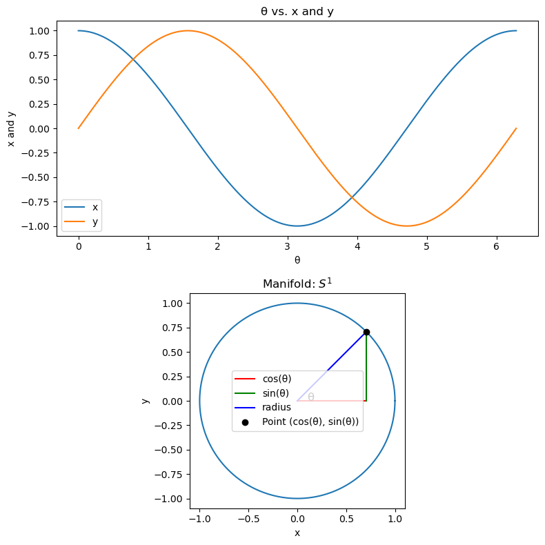
As \(\theta\) varies between 0 and \(2\pi\), the \(x\) and \(y\) values trace out a complete circle. Thus, any point on the circle can be uniquely identified by a single parameter \(\theta\). This demonstrates one of the key properties of a manifold: locally, it behaves just like a simple Euclidean space.
This code and the associated visualization serve as a practical implementation of the manifold concept, offering an intuitive understanding that you can extend to higher-dimensional manifolds. As we proceed, you’ll see that this intuition is crucial to understanding the more complex structures in the realm of Lie Groups. So, keep this circle example in mind as we continue our journey!
This will conclude part 1 of this discussion on the application of Lie Groups to deep learning. In part 2, we’ll explore the concept of a Lie Group, and how it relates to the concept of a manifold. We’ll also explore the concept of a Lie Algebra, and how it relates to the concept of a tangent space. Finally, we’ll explore the concept of a Lie Group action, and how it relates to the concept of a group action.