
HuggingFace Deep RL Course Notes - Unit 1
HuggingFace Deep RL Course Notes
This post is going to be slightly different, as I am going to be using it as a sort of living document to record my notes from the HuggingFace Deep RL Course. I will be updating this post as I work through the course, so check back often for updates!
Unit 1: Introduction to Deep Reinforcement Learning
Note: The Deep in Deep Reinforcement Learning refers to the use of deep neural networks to approximate the agent’s policy \(\pi\) , value function \(V\) , or action-value function \(Q\) . We will explore these concepts in more detail in later units.
We can describe reinforcement learning at a high level via the following process:
- We have an environment \(E\) that is described by a state \(S\) .
- We have an agent \(L\) that can take actions \(A\) in the environment.
- The agent receives a reward \(R\) for each action it takes.
- The agent’s goal is to maximize the total reward it receives.
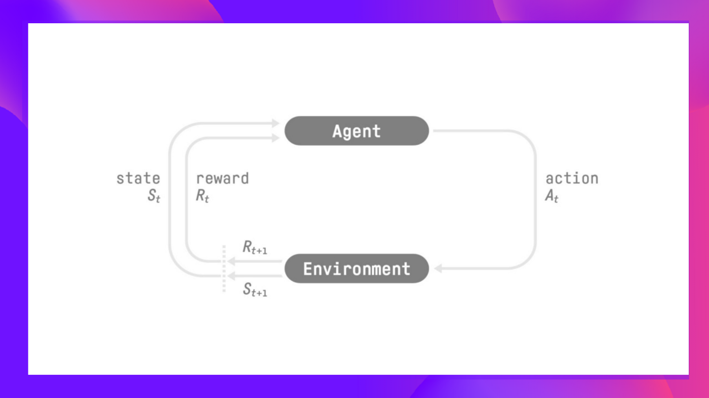
More formally, we can say that an agent first receives an observation \(s_0\) from the environment. The agent then takes an action \(a_0\) based on the observation \(s_0\) . The environment then transitions to a new state \(s_1\) and returns a reward \(r_1\) to the agent. This process repeats until the agent reaches a terminal state.
We can further formalize this even further with the following definitions:
Definitions
Environment
An environment \(E\) is the system or framework within which we are attempting to solve the RL problem.
It can be described by a by a state \(s_t\) at time \(t\) :
\[s_t \in S\]Agent
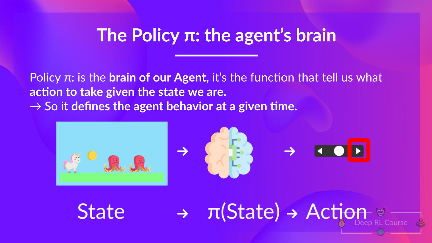
An agent \(L\) is an entity that exists within and interacts with the environment \(E\) . Roughly speaking, the agent \(L\) is the entity that is trying to solve the RL problem. The agent \(L\) is described by a policy \(\pi\) and takes actions \(a_t\) in the environment \(E\).
More formally, the agent is described by a policy \(\pi\) that maps states to actions:
\[L: S \rightarrow A\]That is, given some observation about the current state \(s_t\) , the agent \(L\) will return an action \(a_t\) . This choice is determined by the agent’s policy \(\pi\) .
Policy
A policy \(\pi\) is a function that maps states to actions:
\[\pi: S \rightarrow A\]That is, given some observation about the current state \(s_t\) , the policy \(\pi\) will return an action \(a_t\) . This choice is determined by the agent’s policy \(\pi\) .
Reward
A reward\(r_t\) is a scalar value that the agent receives after taking an action \(a_t\) :
\[r_t \in R\]That is, given some action \(a_t\) , the agent \(L\) will receive a reward \(r_t\) from the environment \(E\) .
Return
The return \(R_t\) is the sum of the rewards that the agent receives after taking an action \(a_t\) :
\[R_t = r_t + r_{t+1} + r_{t+2} + \cdots\]That is, given some action \(a_t\) , the agent \(L\) will receive a reward \(r_t\) from the environment \(E\) . The agent will then take another action \(a_{t+1}\) and receive a reward \(r_{t+1}\) from the environment \(E\) . This process repeats until the agent reaches a terminal state. The return at a given time \(R_t\) is the sum of all of these rewards up to that point.
Discounted Return
The discounted return \(G_t\) is the sum of the rewards that the agent receives after taking an action \(a_t\) , but with each reward discounted by a factor \(\gamma\) :
\[G_t = r_t + \gamma r_{t+1} + \gamma^2 r_{t+2} + \cdots\]That is, given some action \(a_t\) , the agent \(L\) will receive a reward \(r_t\) from the environment \(E\) . The agent will then take another action \(a_{t+1}\) and receive a reward \(r_{t+1}\) from the environment \(E\) . This process repeats until the agent reaches a terminal state. The return at a given time \(R_t\) is the sum of all of these rewards up to that point, but with each reward discounted by a factor \(\gamma\) . This ensures that the more highly probable, early rewards are weighted more heavily than the less probable, later rewards, with respect to the final total return.
This idea is a little bit tricky, so we can take a look at the following figure to get a better intuition for why this needs to be done:
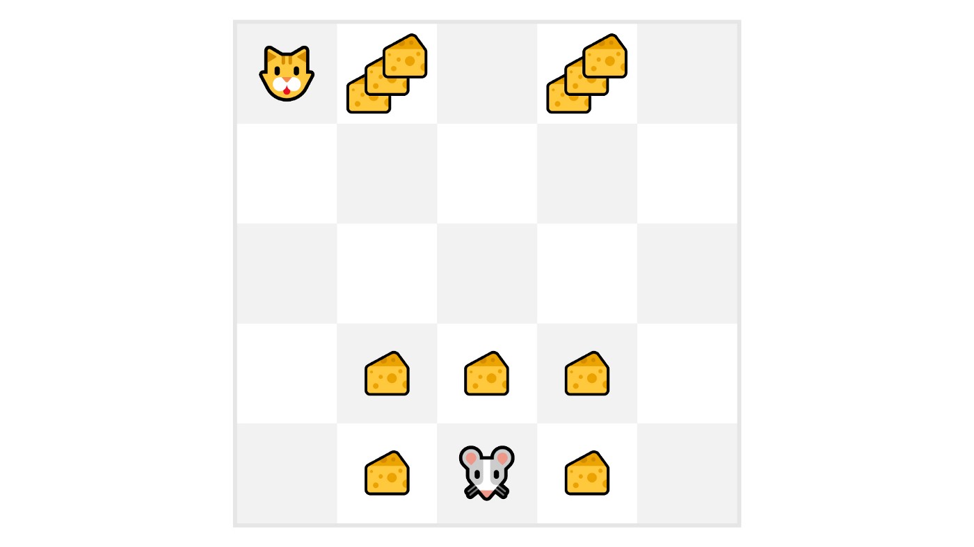
In this figure, we see that our agent (the mouse) has an advesary (the cat). The cat is intially positioned in the top left corner of the grid, and the mouse is positioned in the bottom middle tile. The mouse’s goal is to maximize the amount of cheese it can eat over a given interval before one of the following two events occur:
- The mouse eats all of the cheese
- The cat eats the mouse
The cheese positioned closer to the mouse will need to be weighted higher than the cheese further away, because otherwise our policy might end up causing our agent to get eaten by the cat. This is because the agent will be more likely to get eaten by the cat than it is to eat the cheese further away. This is why we need to discount the rewards that are further away from the agent.
RL-Problem: Finding the Optimal Policy
We can now describe the RL problem as finding the optimal policy \(\pi^*\) that maximizes the return \(R_t\) :
\[\pi^* = \underset{\pi}{\text{argmax}} \sum_{t=0}^{\infty} R_t\]There are two main approaches to solving this problem:
- Value-based methods
- Policy-based methods
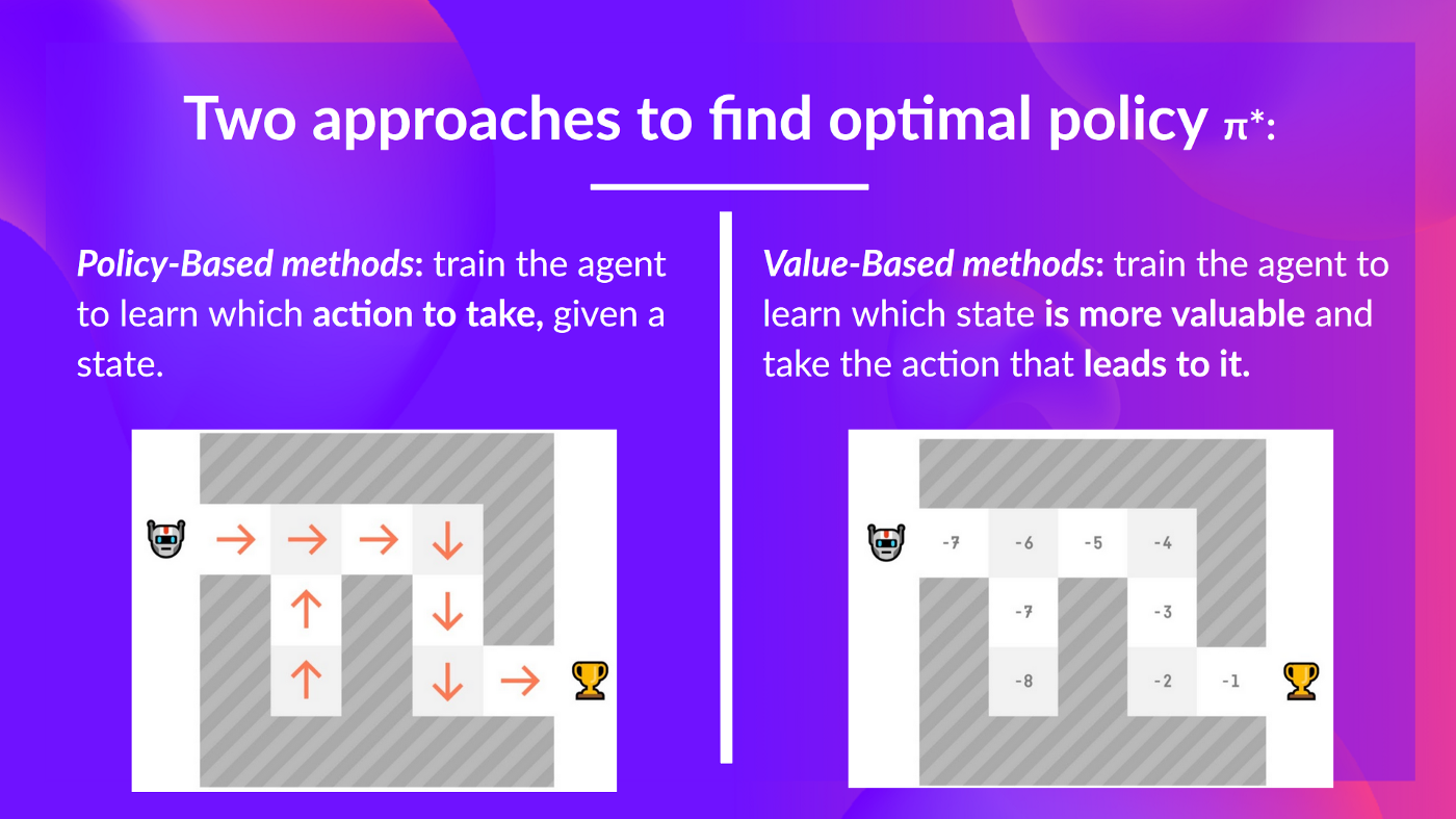
Value-Based Methods
Value-based methods attempt to find the optimal policy \(\pi^*\) by finding the optimal value function \(V^*\) :
\[V^* = \underset{\pi}{\text{argmax}} \sum_{t=0}^{\infty} R_t\]We will explore value-based methods in more detail in the next chapter.
Policy-Based Methods
Policy-based methods attempt to find the optimal policy \(\pi^*\) directly:
\[\pi^* = \underset{\pi}{\text{argmax}} \sum_{t=0}^{\infty} R_t\]We will explore policy-based methods in more detail in later chapters, but for now we can say that policy-based methods have become increasingly popular in recent years given the advancements in deep learning algorithms and capabilities empowered by powerful GPUs, but for this course we are going to start with the foundations via value-based methods and work towards policy-based methods once we have a better grasp on the fundamentals.
Summary
Returning back to what we introduced at the beginning of this unit, we can describe reinforcement learning as the following process:
- We have an environment \(E\) that is described by a state \(S\) .
- We have an agent \(L\) that can take actions \(A\) in the environment.
- The agent receives a reward\(R\) for each action it takes, along with an observation about the new state.
We can state the goal of the agent as maximizing the total reward it receives.
That is, the agent’s goal is to maximize the return \(R_t\) :
\[R_t = r_t + r_{t+1} + r_{t+2} + \cdots\]Therefore our goal will be to find the optimal polciy \(\pi^*\) that maximizes the return \(R_t\) :
\[\pi^* = \underset{\pi}{\text{argmax}} \sum_{t=0}^{\infty} R_t\]We can solve this problem using either value-based methods or policy-based methods.
In the next unit, we will explore value-based methods in more detail through the use of Q-Learning, a popular value-based method for solving RL problems.