
HuggingFace Deep RL Course Notes - Unit 2 (Work in Progress)
Introduction
These post are going to be slightly different, as I am going to be using them as a sort of living document to record my notes from the HuggingFace Deep RL Course. I will be updating this post as I work through the course, so check back often for updates!
You can the notes for Unit 1 here
Thoughts for Potential Projects and Further Areas of Interest
- Are these value functions differentiable? I am assuming so, but since we are dealing with discrete timesteps I am not sure what formulation is needed to take the derivative of these functions. I may be overthinking this, but as we more explicitly define the value functions throughout this unit I am going to keep this question in mind.
Unit 2: Introduction to Q-Learning
In this unit, we will explore Q-Learning, a popular value-based method for solving RL problems.
This will involve us implementing an RL-agent from scratch, in 2 environments:
- Frozen-Lake-v1 (non-slippery version): where our agent will need to go from the starting state (S) to the goal state (G) by walking only on frozen tiles (F) and avoiding holes (H).
- An autonomous taxi: where our agent will need to learn to navigate a city to transport its passengers from point A to point B.
Pulling directly from the course material:
Concretely, we will:
- Learn about value-based methods.
- Learn about the differences between Monte Carlo and Temporal Difference Learning.
- Study and implement our first RL algorithm: Q-Learning. This unit is fundamental if you want to be able to work on Deep Q-Learning: the first Deep RL algorithm that played Atari games and beat the human level on some of them (breakout, space invaders, etc).
So let’s get started! 🚀
For reference, I am including a glosarry of terms and concepts that are either introduced in this unit, or are important to restate here due to their application to the material we will be covering.
Unit 2 - Glossary
Two Types of Value Functions
2.1 State-Value Functions
\[V_{\pi}(s) = \mathbb{E}_{\pi}[R_t | s_t = s]\]2.2 Action-Value Functions
\[Q_{\pi}(s, a) = \mathbb{E}_{\pi}[R_t | s_t = s, a_t = a]\]2.3 Optimal Policy
\[\pi^*(s) = \text{argmax}_{a} Q^*(s, a) \quad \text{for all}\ s\]2.4 Bellman Equation
\[V_{\pi}(s) = \mathbb{E}_{\pi}[R_t | s_t = s] = \mathbb{E}_{\pi}[r_{t+1} + \gamma V_{\pi}(s_{t+1}) | s_t = s]\]$$
2.7/2.8 - Monte-Carlo Learning
\(V(S_t) \leftarrow V(S_t) + \alpha[G_t - V(S_t)]\) \(Q(S_t, A_t) \leftarrow Q(S_t, A_t) + \alpha[G_t - Q(S_t, A_t)]\)
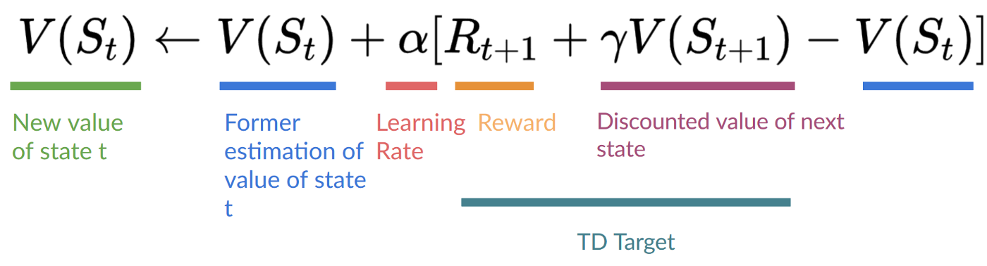
2.9/2.10 Temporal Difference Learning
\(V(S_t) \leftarrow V(S_t) + \alpha[R_{t+1} + \gamma V(S_{t+1}) - V(S_t)]\) \(Q(S_t, A_t) \leftarrow Q(S_t, A_t) + \alpha[R_{t+1} + \gamma Q(S_{t+1}, A_{t+1}) - Q(S_t, A_t)]\)
Unit 2 - Content
Value-Based Methods
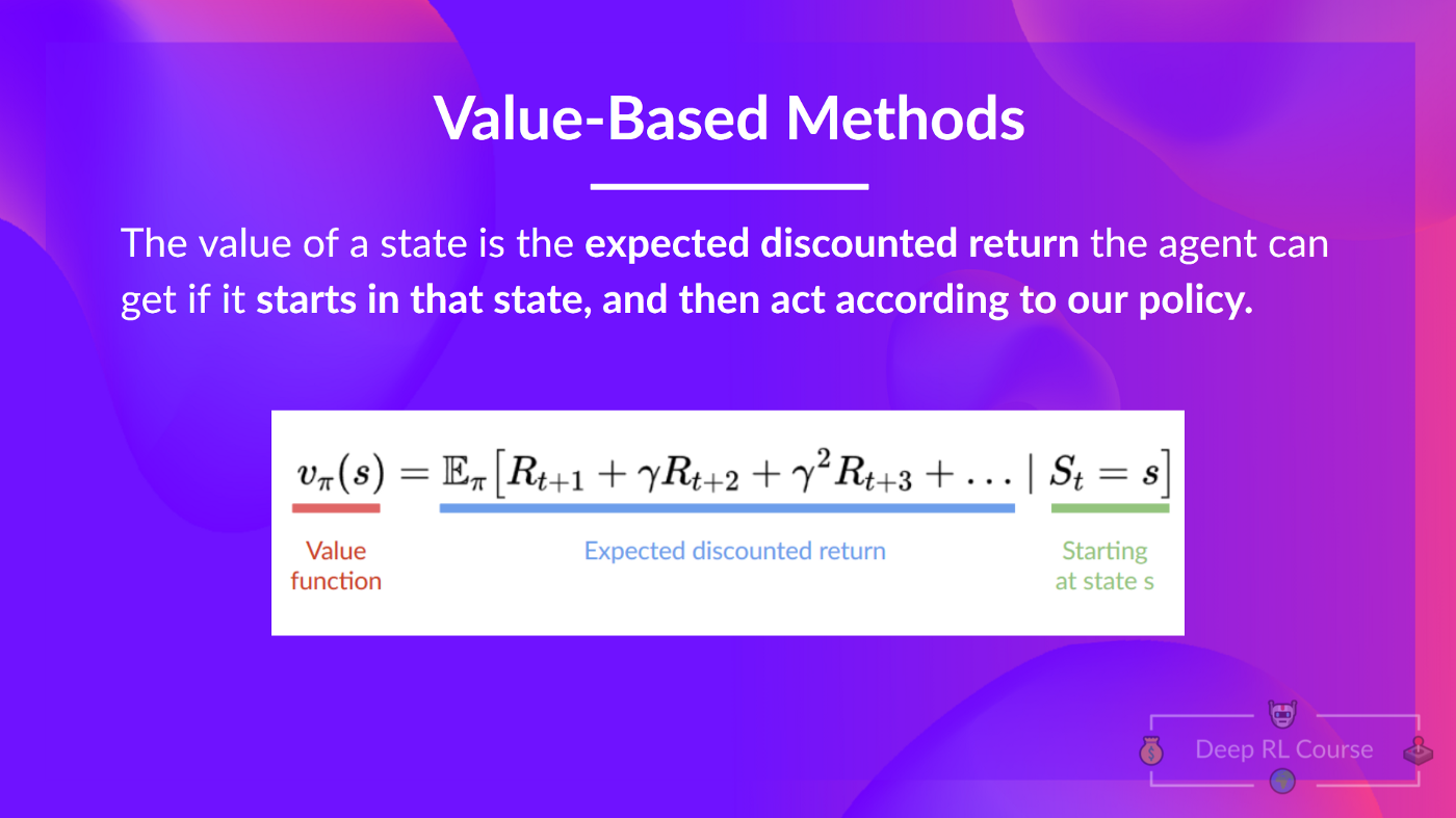
In value-based methods, we learn a value function that maps a state to the expected value of being at that state. This value function is typically denoted as \(V(s)\).
Borrowing directly from HuggingFace:
The value of a state is the expected discounted return the agent can get if it starts at that state and then acts according to our policy.
That is, given some state \(S_t\), the value function \(V(s)\) will return the expected value of being at that state.
Our goal remains the same; we want to find the optimal policy \(\pi^*\) that maximizes the expected return \(G_t\). However, we are not doing so directly, but are instead training a model on a value function for a given state, and define the policy in terms of the value function.
From the course material:
“In fact, most of the time, in value-based methods, you’ll use an Epsilon-Greedy Policy that handles the exploration/exploitation trade-off; we’ll talk about this when we talk about Q-Learning in the second part of this unit.”
Two types of value-based methods
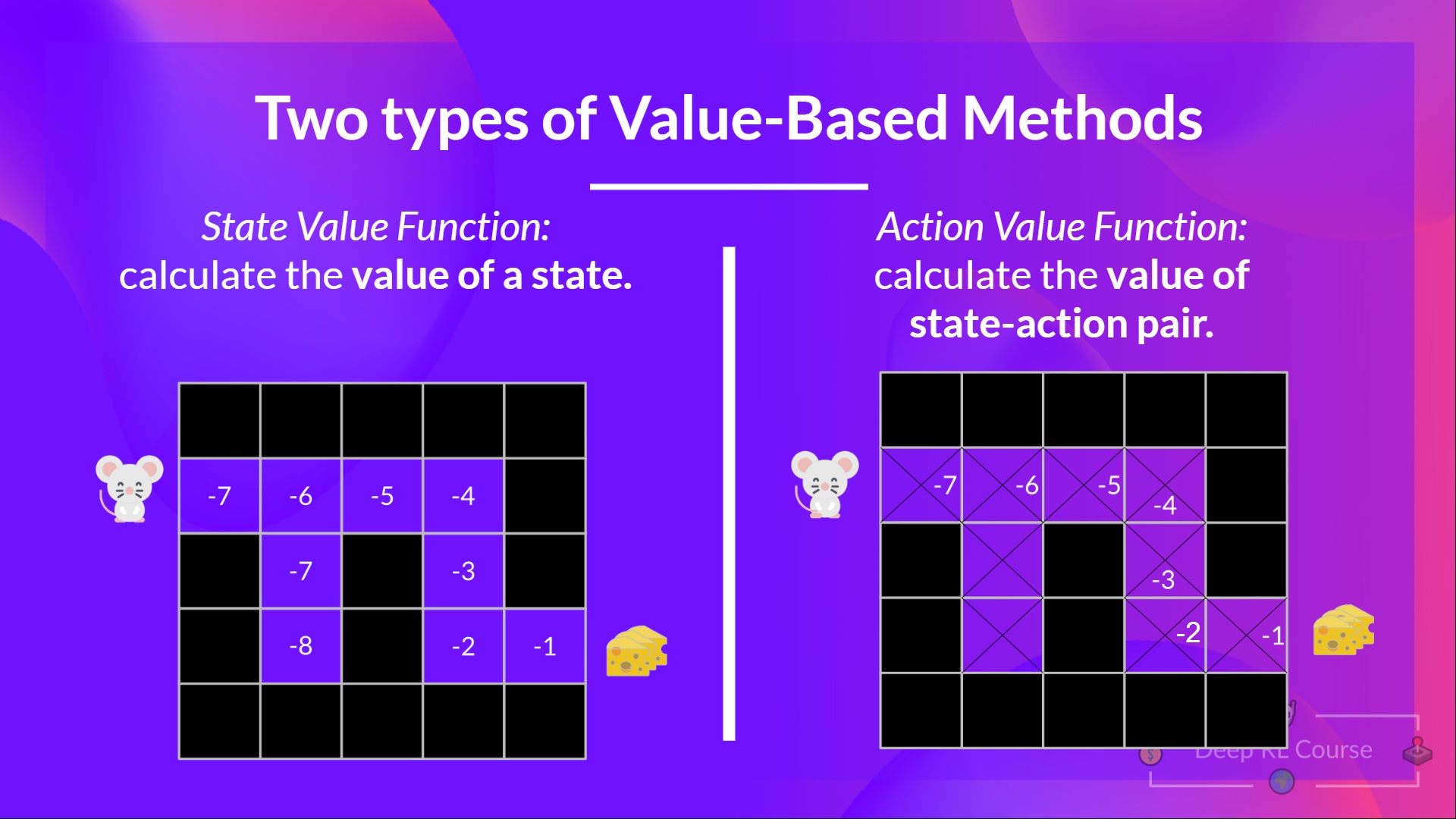
In value-based methods for finding the optimal policy, we have two types of value functions:
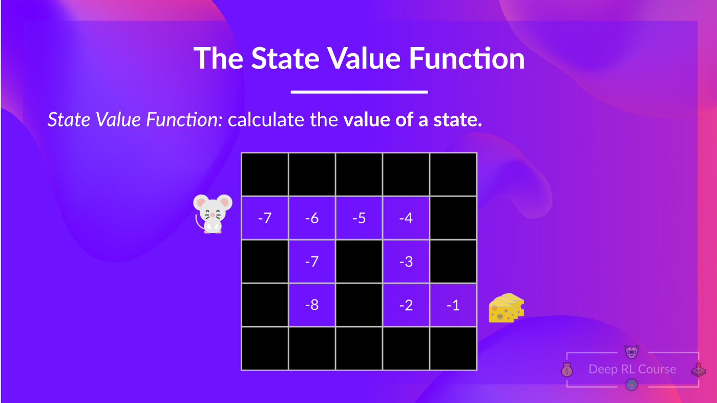
- State-Value Functions
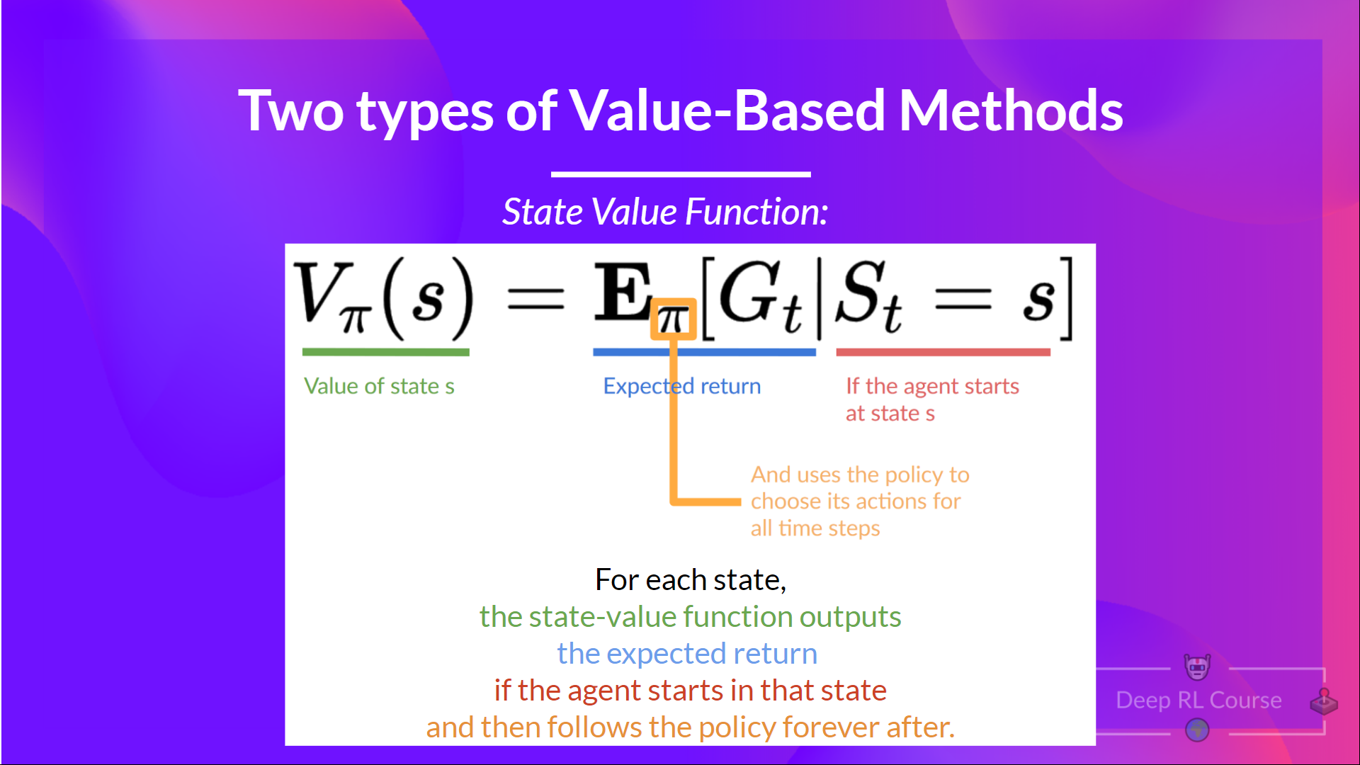
- For the state-value function, we calculate the value of each state \(S_t\),
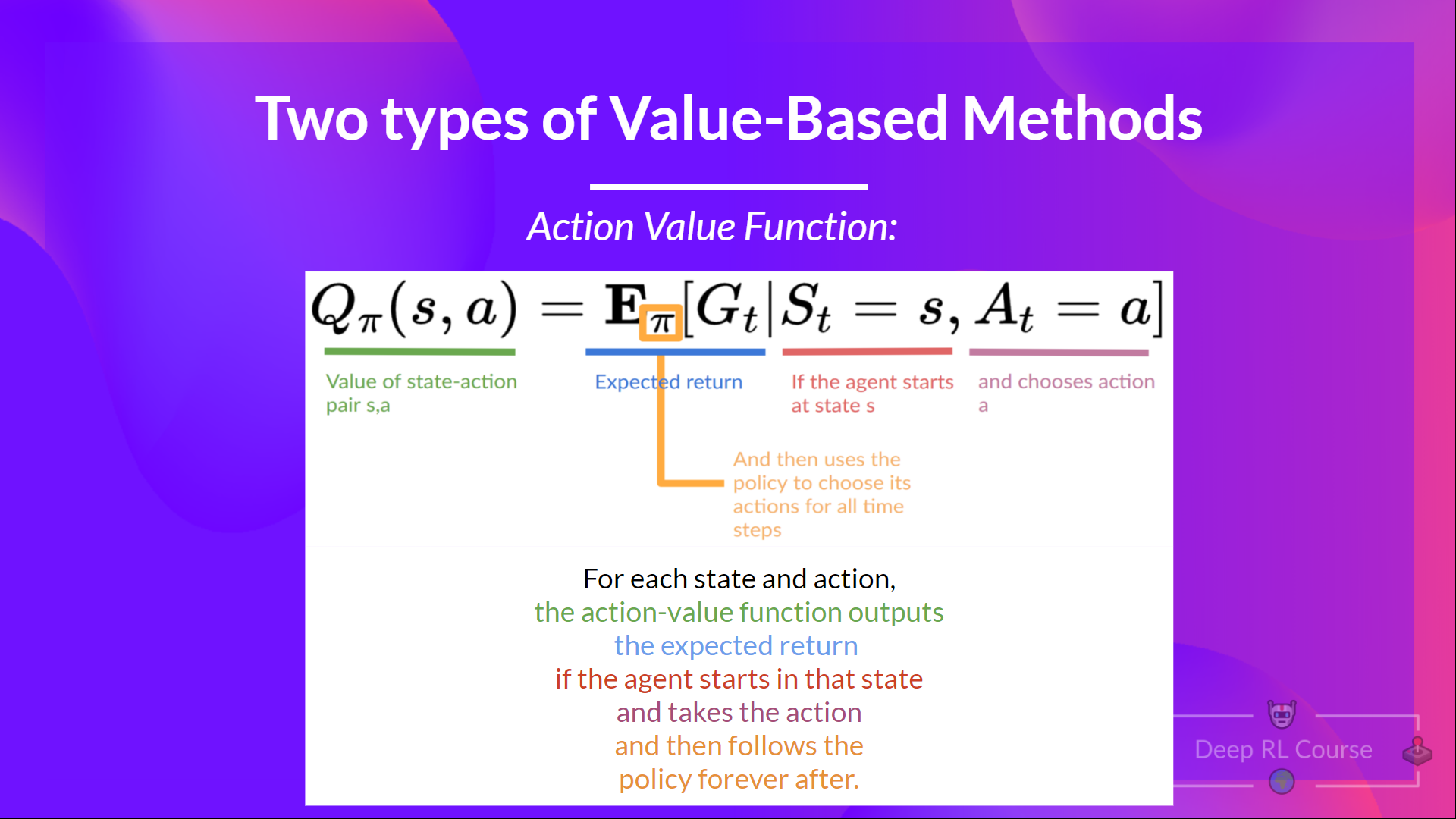
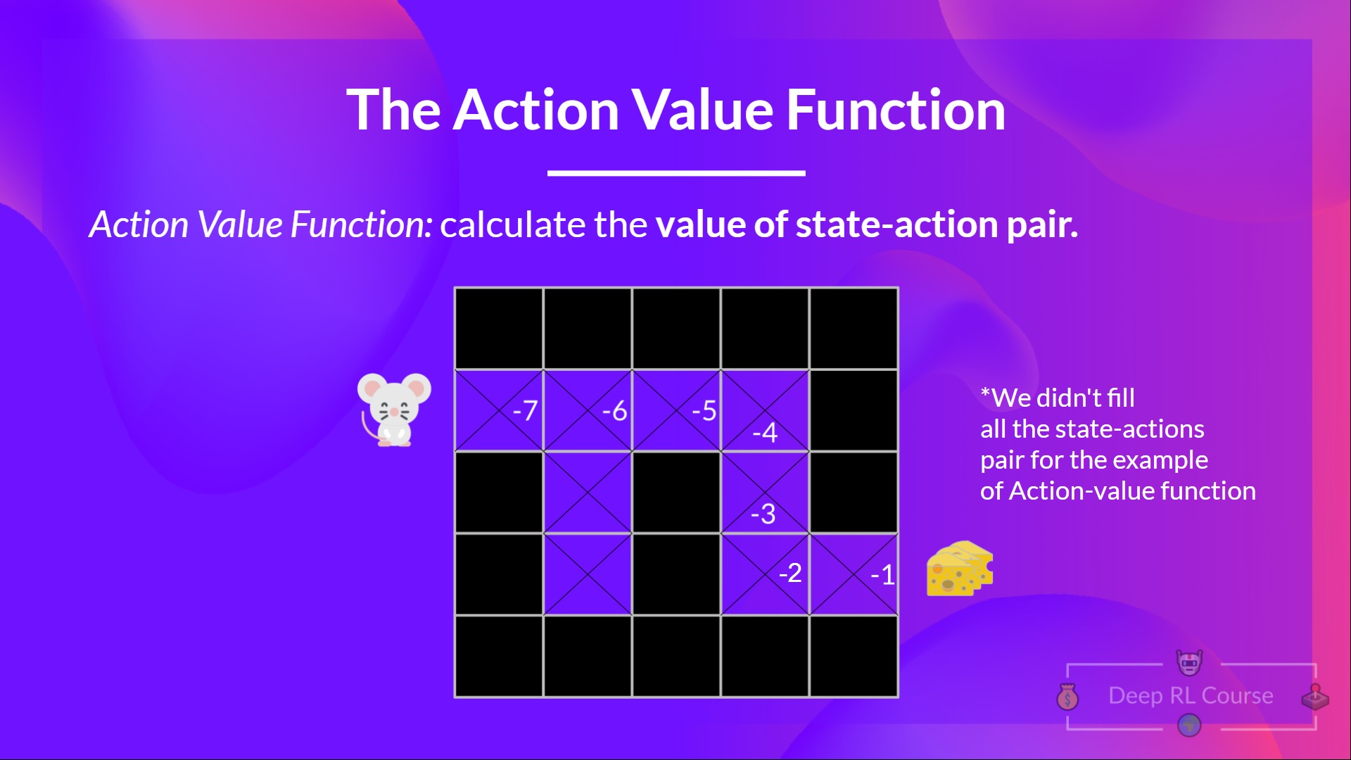
- Action-Value Functions
- For the action-value functions, we assign a value to each tuple \((S_t, A_t)\), where \(A_t\) is the action taken between possible states.
The state-value functions contain less information than the action-value functions, but finding the action-value function explicitly would be much more computationally intensive. Therefore, we are going to introduce our first named equation in the course, the Bellman Equation.
Bellman Equation
We will go ahead and just state the equation, and then we can begin breaking it down and dissecting how exactly it works. For now, just know that it is a recursive function that approximates the computationally expensive state-action-value functions:
\[V_{\pi}(s) = \mathbb{E}_{\pi}[R_t | s_t = s] = \mathbb{E}_{\pi}[r_{t+1} + \gamma V_{\pi}(s_{t+1}) | s_t = s]\]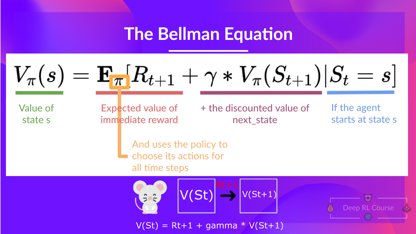
Two Learning Strategies
Monte-Carlo Learning
This type of learning involves looking back after an episode and adjusting the value function based on the actual return.
For a state-value function, we can express this in the following equations:
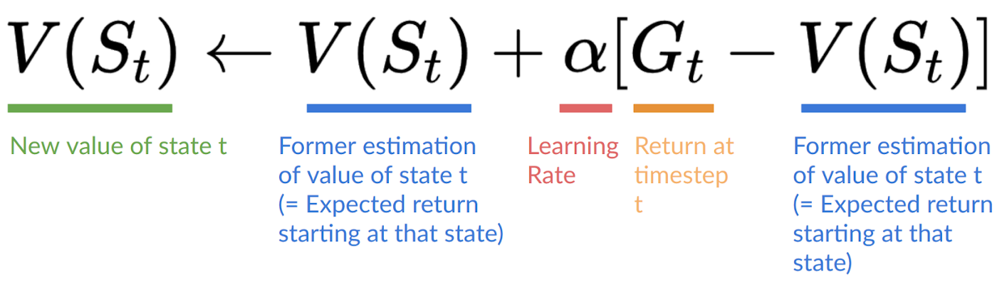
\[V_{\pi}(s) \leftarrow V_{\pi}(s) + \alpha[G_t - V_{\pi}(s)]\]Where here,
- \(G_t\) is the discounted return at time step \(t\)
- \(V_{\pi}(s)\) is the value function, which maps a given state to a certain value.
Then intuitively we can interpret this equation as follows:
- We first play out 1 full episode, and compute the discounted cumulative return, \(G_t\).
- At each timestep \(t\), we adjust the value function by some coefficients \(\alpha\) and the difference between the total return \(G_t\) over the entire episode minus the value function at that state \(V_{\pi}(s)\).
We can see then why we have to wait an entire episode before adjusting the value function for each state \(G_t\). We need to know the total return for the entire episode before we can adjust the value function for each state. The amount by which each state is adjusted by the amount it didn’t contribute to \(G_t\), scaled by a coefficient \(\alpha\). So that highest values for each of the states will be adjusted less than the ones that contributed the least to \(G_t\). The factor \(\alpha\) is the learning rate, and adds an additional parametrizable constraint we can adjust in order to achieve our ultimate goal of finding the optimal policy \(\pi^*\).
Extending this to the state-action-value function \(Q_{\pi}(s, a)\), we can express the Monte-Carlo learning equation as follows:
\[Q_{\pi}(s, a) \leftarrow Q_{\pi}(s, a) + \alpha[G_t - Q_{\pi}(s, a)]\]Where here the parameters of this equation follow naturally from the parameters we defined for the state-value function \(V_{\pi}(s)\).
Going back to a state-value function \(V_{\pi}(S_t)\), we will borrow some nice summarization and illustration from the Hugging Face course:
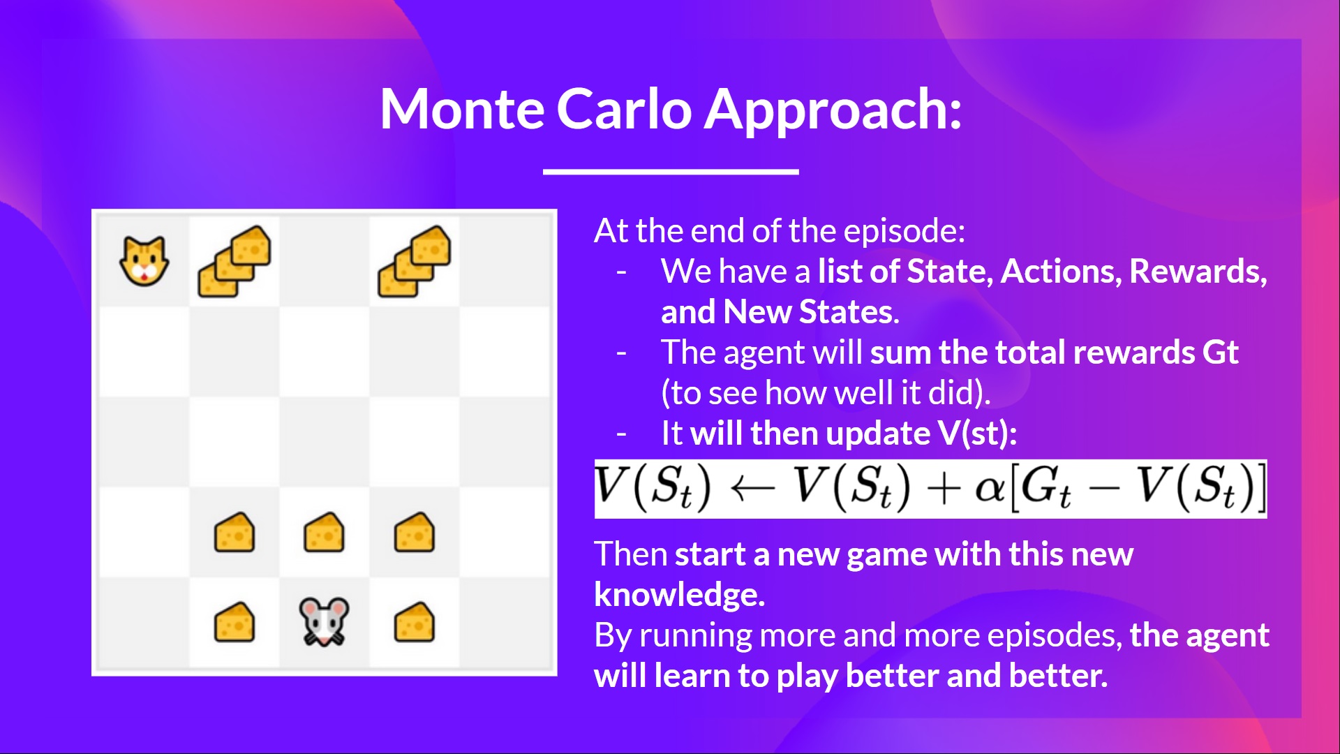
Example of Monte-Carlo Learning
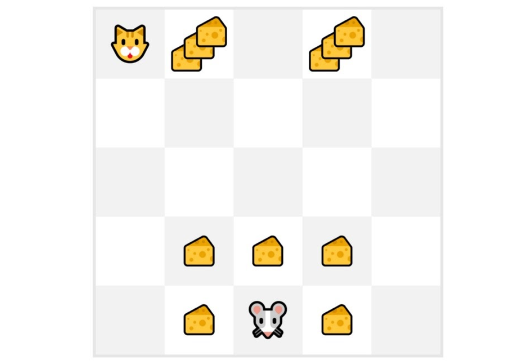
- We will always start each episode at the same starting point
- The agent takes actions using the policy. For instance, using an Epsilon Greedy Strategy, a policy that alternates between exploration (random actions) and exploitation.
- We get the reward and the next state.
- We terminate the episode if the cat eats the mouse or if the mouse moves > 10 steps.
- At the end of the episode, we have a list of State, Actions, Rewards, and Next States tuples For instance [[State tile 3 bottom, Go Left, +1, State tile 2 bottom], [State tile 2 bottom, Go Left, +0, State tile 1 bottom]…]
- The agent will sum the total rewards \(G_t\) (to see how well it did).
- It will then update \(V(S_t)\) based on the formula
- The agent will then start a new episode and repeat the process.
- The process can be summarized by the following illustration:
Now, we will move onto a more scalable solution, Temporal Difference Learning.
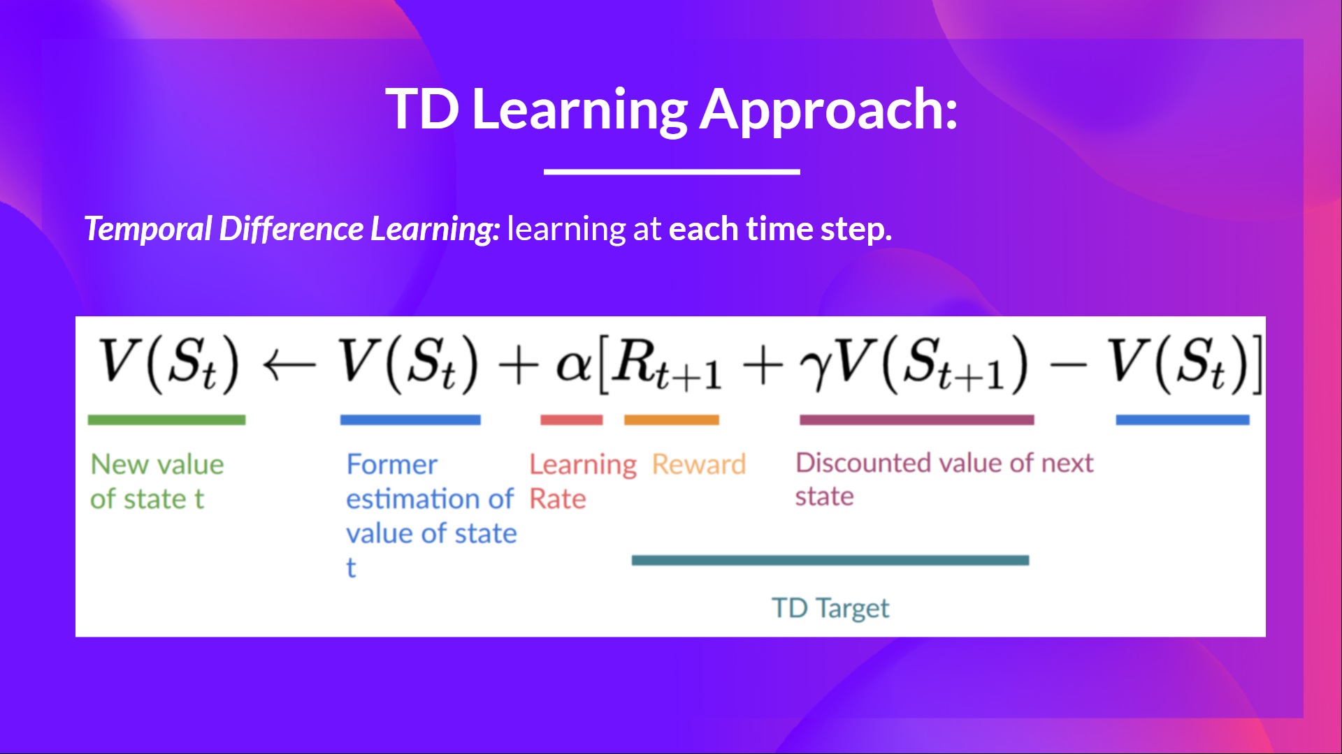
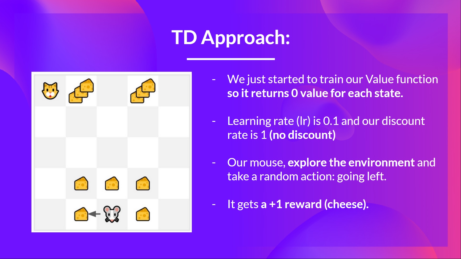
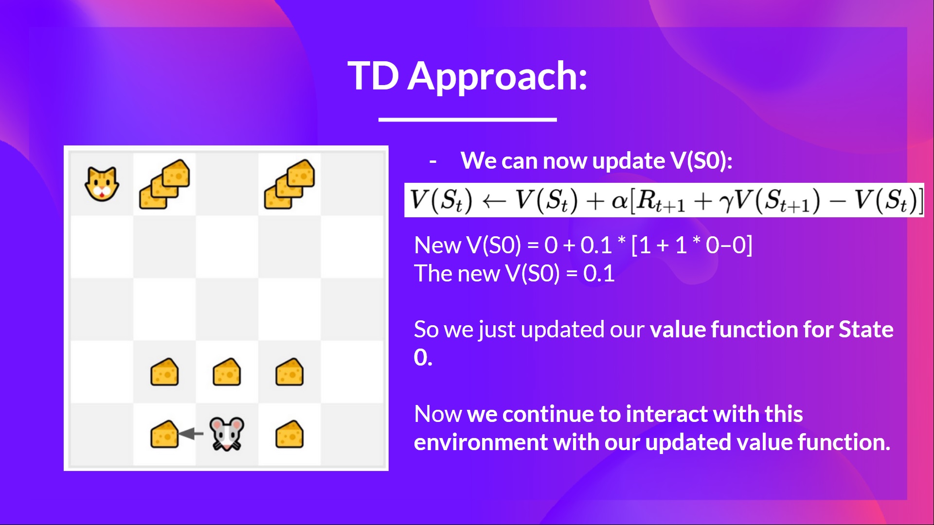
Temporal Difference Learning
In contrast with Monte-Carlo Learning, where we must wait an entire episode before adjusting the value function, in Temporal Difference Learning we only need a single timestep \(t\) before we adjust our value function:

Introducing Q-Learning
What is Q-Learning? Q-Learning is an off-policy value-based method that uses a TD approach to train its action-value function:
- Off-policy: we’ll talk about that at the end of this unit.
- Value-based method: finds the optimal policy indirectly by training a value or action-value function that will tell us the value of each state or each state-action pair.
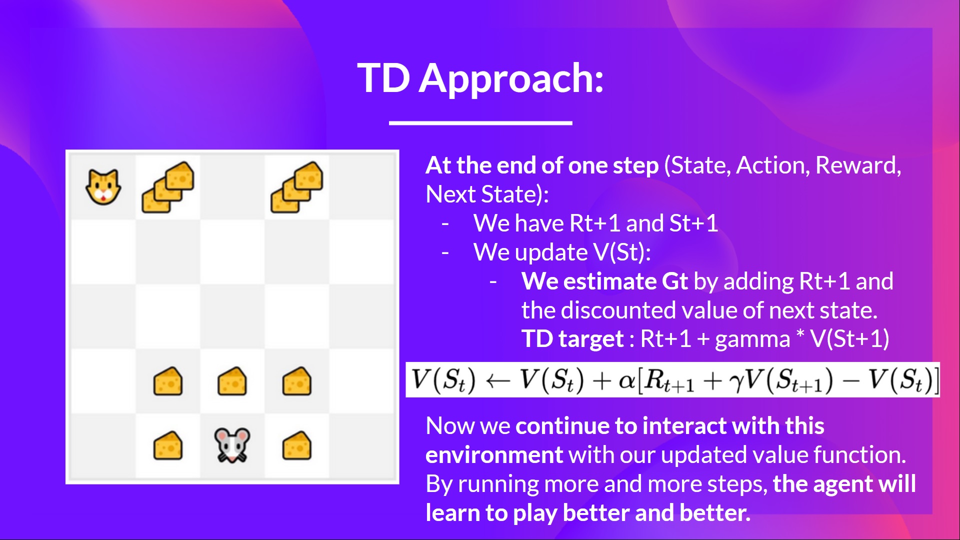
- TD approach: updates its action-value function at each step instead of at the end of the episode.
- Q-Learning is the algorithm we use to train our Q-function, an action-value function that determines the value of being at a particular state and taking a specific action at that state.
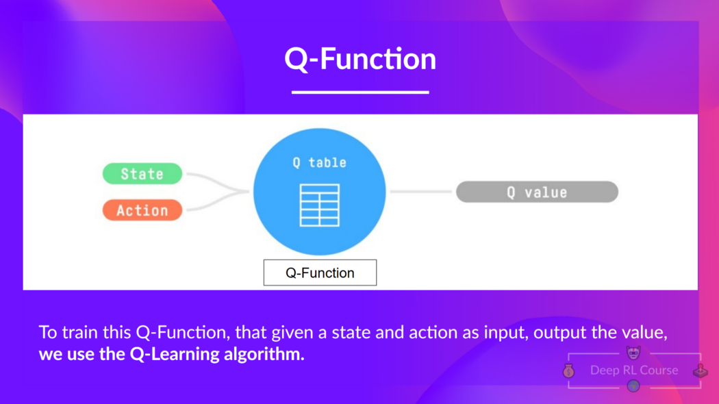
Q-table
to be continued…